Poisson distribution

Poisson distribution
	Probability mass function The horizontal axis is the index k, the number of occurrences. λ is the expected rate of occurrences. The vertical axis is the probability of k occurrences given λ. The function is defined only at integer values of k; the connecting lines are only guides for the eye.
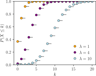
	Cumulative distribution function The horizontal axis is the index k, the number of occurrences. The CDF is discontinuous at the integers of k and flat everywhere else because a variable that is Poisson distributed takes on only integer values.
Notation
Parameters	(rate)
Support	(Natural numbers starting from 0)
PMF
CDF	or or (for where is the upper incomplete gamma function, is the floor function, and is the regularized gamma function)
Mean
Median
Mode
Variance
Skewness
Excess kurtosis
Entropy	or for large
MGF
CF
PGF
Fisher information

In probability theory and statistics, the Poisson distribution (/ˈpwɑːsɒn/) is a discrete probability distribution that expresses the probability of a given number of events occurring in a fixed interval of time if these events occur with a known constant mean rate and independently of the time since the last event.^[1] It can also be used for the number of events in other types of intervals than time, and in dimension greater than 1 (e.g., number of events in a given area or volume). The Poisson distribution is named after French mathematician Siméon Denis Poisson. It plays an important role for discrete-stable distributions.

Under a Poisson distribution with the expectation of λ events in a given interval, the probability of k events in the same interval is:^[2]^: 60

{\frac {\lambda ^{k}e^{-\lambda }}{k!}}.

For instance, consider a call center which receives an average of λ = 3 calls per minute at all times of day. If the calls are independent, receiving one does not change the probability of when the next one will arrive. Under these assumptions, the number k of calls received during any minute has a Poisson probability distribution. Receiving k = 1 to 4 calls then has a probability of about 0.77, while receiving 0 or at least 5 calls has a probability of about 0.23.

A classic example used to motivate the Poisson distribution is the number of radioactive decay events during a fixed observation period.^[3]

^ Cite error: The named reference Haight1967 was invoked but never defined (see the help page).
^ Cite error: The named reference Yates2014 was invoked but never defined (see the help page).
^ Ross, Sheldon M. (2014). Introduction to Probability Models (11th ed.). Academic Press.

[Haight1967-1] Cite error: The named reference Haight1967 was invoked but never defined (see the help page).

[Yates2014-2] Cite error: The named reference Yates2014 was invoked but never defined (see the help page).

[3] Ross, Sheldon M. (2014). Introduction to Probability Models (11th ed.). Academic Press.

[1]

[2]

[3]

Probability mass function The horizontal axis is the index $k$ , the number of occurrences. $λ$ is the expected rate of occurrences. The vertical axis is the probability of $k$ occurrences given $λ$ . The function is defined only at integer values of $k$ ; the connecting lines are only guides for the eye.
Cumulative distribution function The horizontal axis is the index $k$ , the number of occurrences. The CDF is discontinuous at the integers of $k$ and flat everywhere else because a variable that is Poisson distributed takes on only integer values.
Notation	$\operatorname {Pois} (\lambda )$
Parameters	$\lambda \in (0,\infty )$ (rate)
Support	$k\in \mathbb {N} _{0}$ (Natural numbers starting from 0)
PMF	${\frac {\lambda ^{k}e^{-\lambda }}{k!}}$
CDF	${\frac {\Gamma (\lfloor k+1\rfloor ,\lambda )}{\lfloor k\rfloor !}},$ or $e^{-\lambda }\sum _{j=0}^{\lfloor k\rfloor }{\frac {\lambda ^{j}}{j!}},$ or $Q(\lfloor k+1\rfloor ,\lambda )$ (for $k\geq 0,$ where $\Gamma (x,y)$ is the upper incomplete gamma function, $\lfloor k\rfloor$ is the floor function, and $Q$ is the regularized gamma function)
Mean	$\lambda$
Median	$\approx \left\lfloor \lambda +{\frac {1}{3}}-{\frac {1}{50\lambda }}\right\rfloor$
Mode	$\left\lceil \lambda \right\rceil -1,\left\lfloor \lambda \right\rfloor$
Variance	$\lambda$
Skewness	${\frac {1}{\sqrt {\lambda }}}$
Excess kurtosis	${\frac {1}{\lambda }}$
Entropy	$\lambda {\Bigl [}1-\log(\lambda ){\Bigr ]}+e^{-\lambda }\sum _{k=0}^{\infty }{\frac {\lambda ^{k}\log(k!)}{k!}}$ or for large $\lambda$ ${\begin{aligned}\approx {\frac {1}{2}}\log \left(2\pi e\lambda \right)-{\frac {1}{12\lambda }}-{\frac {1}{24\lambda ^{2}}}\\-{\frac {19}{360\lambda ^{3}}}+{\mathcal {O}}\left({\frac {1}{\lambda ^{4}}}\right)\end{aligned}}$
MGF	$\exp \left[\lambda \left(e^{t}-1\right)\right]$
CF	$\exp \left[\lambda \left(e^{it}-1\right)\right]$
PGF	$\exp \left[\lambda \left(z-1\right)\right]$
Fisher information	${\frac {1}{\lambda }}$

Poisson distribution

From Wikipedia, the free encyclopedia · View on Wikipedia